Passive Low-Pass Filter Circuit Design & Cutoff Calculation
Designing a passive low-pass filter (LPF) is a fundamental skill in analog hardware engineering, sensor signal conditioning, and high-fidelity audio system development. Unlike active filters that rely on operational amplifiers or operational transistors to supply gain, passive topologies leverage discrete, non-powered electrical components to smoothly attenuate high-frequency noise while allowing lower frequency spectrum waveforms to pass unobstructed. In advanced automation nodes, implementing localized low-pass filtering shields communication tracks against electromagnetic interference (EMI) generated by high-power residential switches or motor controllers.
This engineering manual outlines the mathematical equations for first-order RC filters, precise component sizing workflows, and benchtop oscilloscope verification protocols.
Core Circuit Engineering Thresholds
Before calculating your capacitive and resistive thresholds, establish your analog processing parameters:
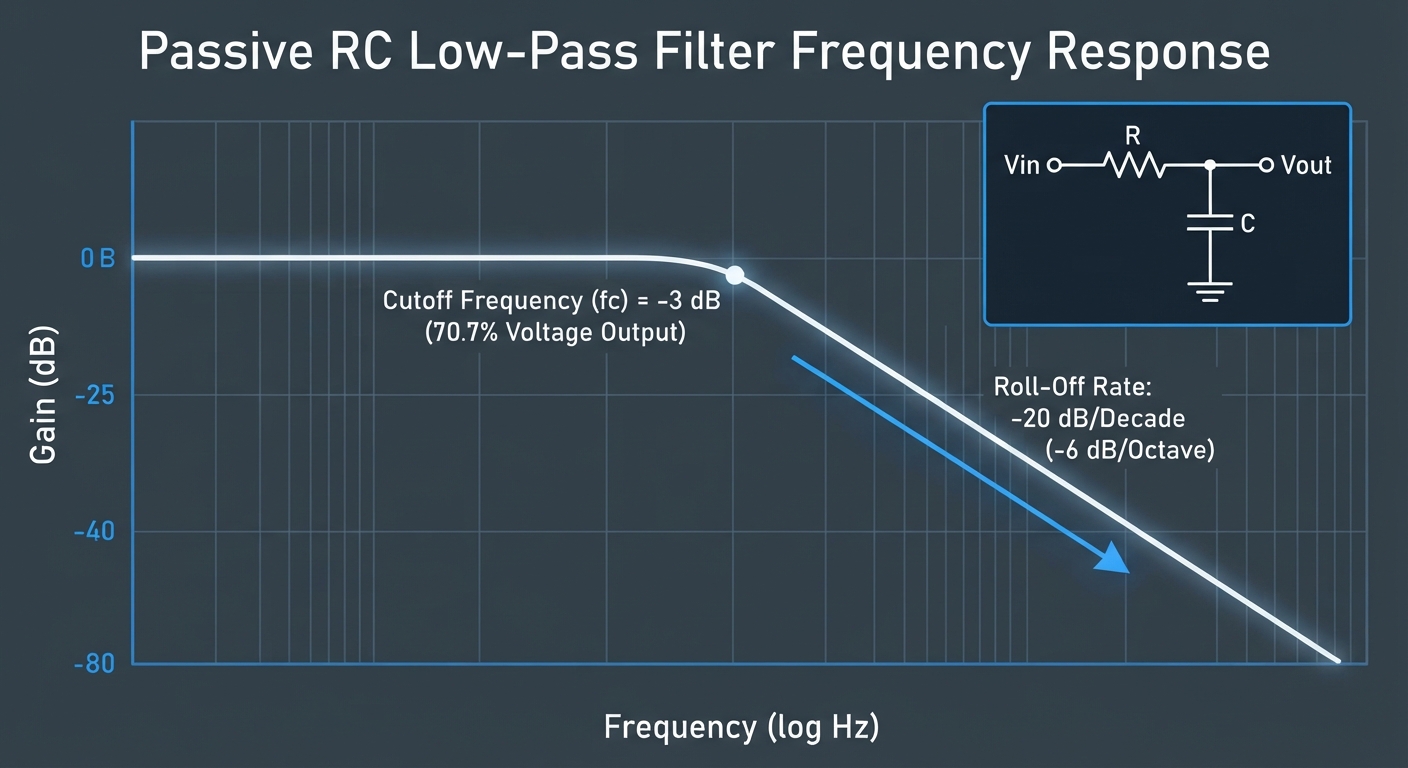
- The Cutoff Point (fc): Also known as the half-power or -3 dB point, this is the exact frequency coordinates where the output signal voltage drops to 70.7% of the original input voltage profile.
- The Insertion Loss Factor: Because passive components lack external DC power supply loops, they inherently introduce a minor voltage attenuation within the desired passband due to internal resistor tolerances.
- Impedance Matching Constraints: The output impedance of your passive filter circuit must interface cleanly with the input impedance of the downstream stage to avoid loading effects that alter the calculated cutoff parameters.
Technical Materials & Laboratory Testing Checklist
Executing, simulating, and auditing micro-electronic signal filters requires precise benchtop instrumentation distinct from heavy building service equipment:
| Electronics Lab Instrument | Primary Engineering Purpose |
|---|---|
| Solderless Breadboard Loop | Allows rapid prototyping and real-time swap-outs of trial resistors and capacitors. |
| Digital Function Generator | Emits precise sine, square, and triangle wave frequencies (1 Hz to 20 MHz) into the filter input. |
| Digital Storage Oscilloscope | Compares the input vs. output phase shifts and visualizes high-frequency attenuation dropouts. |
| Precision LCR Multimeter | Measures exact internal component tolerances down to picofarads (pF) and fractional Ohms (Ω). |
| ESD-Safe Temperature Iron | Formulates low-resistance alloy joints on copper prototype printed circuit boards (PCBs). |
The Mathematics of the Cutoff Frequency: First-Order RC Equations
The structural response of a first-order passive low-pass filter relies entirely on the frequency-dependent behavior of capacitive reactance (XC). As input signal frequencies rise, the internal resistance impedance of the capacitor drops, effectively shunting high-frequency noise tracks directly to the system ground line.
To determine the exact mathematical intersection where your passband transitions into the attenuation slope, apply the standard RC time-constant formula:
fc = 1 / (2 × π × R × C)
Where:
- fc = Cutoff frequency measured strictly in Hertz (Hz).
- R = Core filter resistance measured in Ohms (Ω).
- C = Core filter capacitance measured in Farads (F).
Passive RC Filter Frequency Response Curve
Practical Engineering Example: Sizing an Audio Filter Loop
Suppose you are designing an inline noise filter for a smart automation audio intercom node to suppress high-frequency digital switching hum lines above 1.2 kHz (1,200 Hz).
-
Rearrange the mathematical equation to solve for the combined RC time constant product parameter:
R × C = 1 / (2 × π × 1200) ≈ 132.62 × 10⁻⁶ seconds (132.62 µs)
-
Select a standard, highly available resistor value from your lab kit. Opting for a 1.5 kΩ resistor (1,500 Ω) with a tight 1% tolerance profile, calculate the matching capacitor parameter requirement:
C = 132.62 × 10⁻⁶ / 1500 ≈ 88.41 × 10⁻⁹ F ───> 88.4 nF
Since 88.4 nF is not a standard manufactured value, a hardware engineer will deploy a standard 82 nF or 100 nF ceramic disc capacitor and fine-tune the low-end trim potentiometer to lock the circuit into the exact target frequency window.
Frequency Response, Roll-Off Rates & Attenuation Decades
A first-order passive RC low-pass filter provides a fixed attenuation slope once the signal frequency crosses the fc threshold coordinates. Understanding this rate of signal decay is critical for mapping noise-rejection parameters.
The -20 dB per Decade Rule
Because a first-order filter incorporates a single reactive component (one capacitor), its maximum theoretical roll-off rate is structurally limited:
- Decade Slope: The circuit attenuates high-frequency noise at a rate of -20 dB per decade (every time the frequency multiplies by 10, the signal power drops by 99%).
- Octave Slope: This translates precisely to a roll-off rate of -6 dB per octave (every time the signal frequency doubles, the voltage output halves).
Multi-Stage Cascading Limitations
If your signal conditioning requirements demand a steeper roll-off profile (such as -40 dB or -60 dB per decade to protect high-frequency processing lanes), multiple RC stages can be cascaded in series. However, cascading passive stages introduces immediate impedance loading degradation. For advanced automation modules requiring active signal isolation between stages, review our detailed guide on BJT transistor switching and amplification manuals to isolate circuit loops flawlessly.
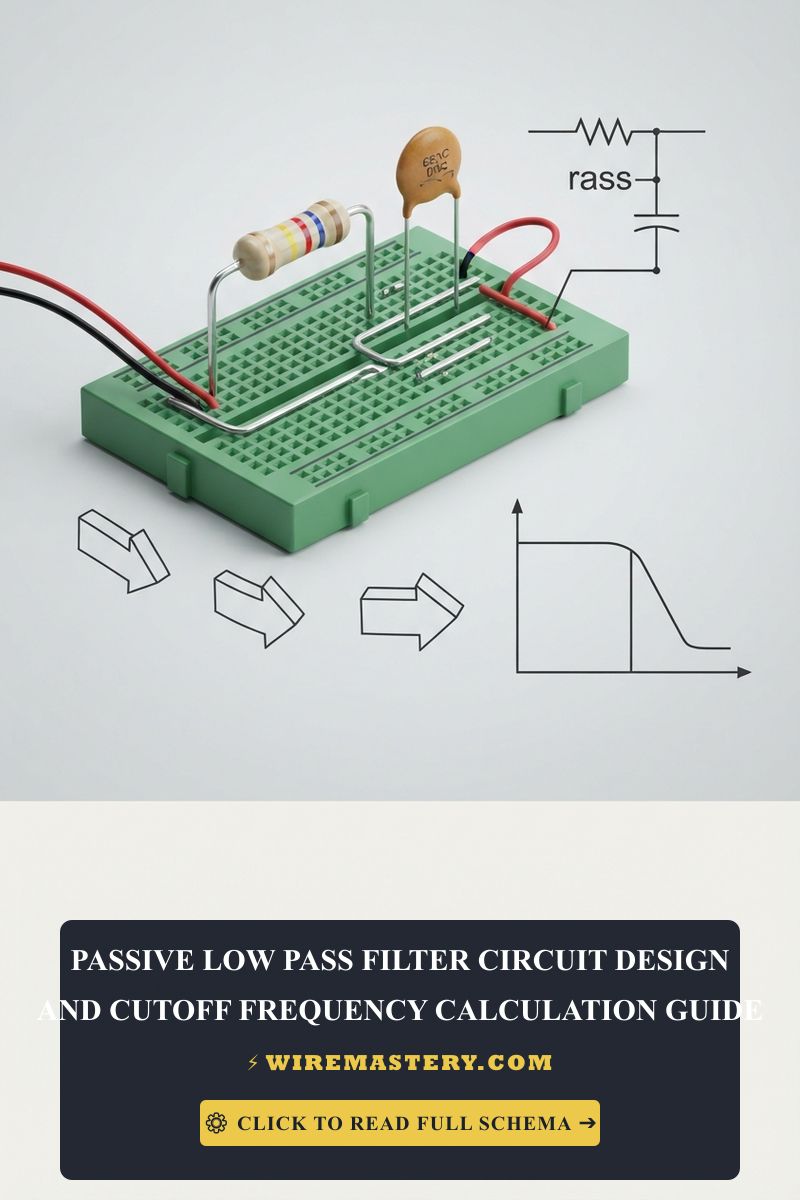
🛠️ Signal Integrity Verification Note: Look closely at the realistic schematic layouts and high-frequency testing diagrams displayed across your guide frameworks. Notice that signal processing traces require ultra-short track geometries. When prototyping high-frequency circuits on solderless breadboards, stray capacitive coupling between adjacent spring-clip rows can introduce up to 5pF of parasitic capacitance, which shifts your calculated cutoff frequency parameters. Always transition to a permanent copper PCB layout to lock in calibration metrics.
Step-by-Step Bench Prototyping & Testing Blueprint
1. Circuit Assembly on a Solderless Breadboard
Insert your chosen tight-tolerance 1.5 kΩ resistor and 88.4 nF capacitor (or standard equivalents) into the breadboard terminal strips. Connect the input signal wire line to one side of the resistor. Tie the opposing side of the resistor to the positive leg of the capacitor. Route the negative leg of the capacitor directly back to the common system ground rail.
2. Splicing Low-Voltage Conductor Leads
For low-power analog communication and signal conditioning loops operating below 1 Amp, utilize 22 AWG solid copper jumper wires hookup leads. Avoid using thick residential wire sizes like 14 AWG or 12 AWG, as heavy solid copper leads will distort or physically damage miniature micro-component prototyping blocks.
3. Executing Waveform Verification with an Oscilloscope
- Connect the output clamp of your digital function generator to the input rail of the filter loop. Set the wave output to a clean 1V Peak-to-Peak (V_pp) sine wave.
- Clip the Channel 1 probe of your digital storage oscilloscope to the filter input node and the Channel 2 probe directly across the capacitor (the output node).
- Sweep the frequency from 100 Hz up to 10 kHz. Observe the Channel 2 display panel closely; as the generator approaches your calculated 1.2 kHz cutoff coordinate, the output wave amplitude will shrink precisely down to 0.707V (V_pp), and the signal phase shift will lock exactly at a 45-degree lag.
Troubleshooting Common Analog Filtering Failures
- The Cutoff Frequency is Drastically Shifted: This behavior indicates component tolerance errors or parasitic circuit resistance. Always audit your capacitors using a precision LCR multimeter before soldering. Standard ceramic disc capacitors frequently carry a ±20% manufacturer tolerance, which can shift a calculated 1.2 kHz cutoff layout deep into the 1.5 kHz or 900 Hz brackets.
- High-Frequency Noise Bleeds through the Filter Completely: Check for a compromised or high-impedance ground path loop. If your capacitor’s ground track is narrow, long, or unbonded, the inductive resistance creates a voltage barrier that blocks high-frequency signals from shunting to ground, rendering the low-pass filter useless.
- The Output Signal Suffers Massive DC Voltage Attenuation: This indicates heavy circuit loading. If the downstream component’s input impedance is too low relative to your filter’s resistor value, it creates a voltage divider loop that crushes your passband signal amplitude before it ever reaches the processing chip.
National Electrical Code Infrastructure & Isolation Context
While individual Class 2 low-voltage analog electronic filters operating below 30V AC / 60V DC are exempt from regional municipal branch inspections, any micro-automation circuit that interfaces with building infrastructure must comply with the strict separation rules of the National Electrical Code (NEC).
Under NEC Article 725 (Remote-Control, Signaling, and Power-Limited Circuits), all low-voltage signal conditioning and data cables must maintain a minimum 2-inch clear physical separation from high-voltage 120V/240V residential power branch lines inside wall cavities and junction enclosures. This isolation prevents dangerous line-voltage electromagnetic induction or arcing from crossing into low-voltage automation boards and burning out sensitive semiconductor layers.
For current NFPA 70 guidance relevant to powered filter equipment, enclosure wiring, grounding, and installation safety, consult the Official NFPA 70: National Electrical Code (NEC).
Conclusion
This guide covers calculating component tolerances and deploying a passive low-pass filter circuit steps up your analog troubleshooting capabilities and secures crisp signal integrity across your home automation systems. By mastering the RC time-constant equation (fc = 1 / (2 × π × R × C)), mapping out standard roll-off rates, and enforcing strict NEC code isolation boundaries against high-voltage lines, you construct highly resilient, electronic networks. Prioritize benchtop function generator testing validation, eliminate high-impedance grounding paths, and design every signal loop with systematic precision.